A polling firm asks 600 adults two questions: how old are you, and where do you get most of your news? Each answer is a category, not a number, so neither a mean nor a scatterplot helps. The question worth asking is whether the answer to one depends on the answer to the other: do younger adults get their news from different places than older adults? Answering it takes a table and a graph built for two categorical variables at once.
Two-way tables
A two-way table (also called a contingency table) sorts every individual by two categorical variables at the same time. One variable's categories label the rows, the other's label the columns, and each cell holds the individuals who fall in that row and that column. Here are the poll's results:
| Age group | Social media | Television | News website or app | Total |
|---|---|---|---|---|
| 18 to 34 | 110 | 30 | 60 | 200 |
| 35 to 54 | 54 | 54 | 72 | 180 |
| 55 and over | 33 | 132 | 55 | 220 |
| Total | 197 | 216 | 187 | 600 |
Read a cell as a sentence: 132 of the 600 adults are 55 or older and get most of their news from television. The row totals give the distribution of age by itself (200, 180, 220), the column totals give the distribution of news source by itself (197, 216, 187), and both sets of totals add to the grand total, 600. That last fact is your arithmetic check every time you fill in or read a table.
The cells can hold counts (frequencies), as above, or proportions (relative frequencies), such as each count divided by 600 or by its row total. Which proportions you compute changes what the table says; topic 2.2 names the three kinds (joint, marginal and conditional) and computes each.
A table of counts answers "how many" questions directly, but it hides the comparison you usually care about. The three age groups have different sizes, so 54 social-media users means something different out of 180 people than out of 220. To compare groups fairly, convert each group's counts to proportions of that group. Divide each row by its own total:
| Age group | Social media | Television | News website or app | Total |
|---|---|---|---|---|
| 18 to 34 | 0.55 | 0.15 | 0.30 | 1.00 |
| 35 to 54 | 0.30 | 0.30 | 0.40 | 1.00 |
| 55 and over | 0.15 | 0.60 | 0.25 | 1.00 |
Each row is now the distribution of news source within one age group, and the rows can be compared directly: 55% of the youngest group lean on social media, against 15% of the oldest.
Three graphs for two categorical variables
All three graphs below follow the same plan: for each category of one variable, show how the individuals in it split across the categories of the other. They differ in what the bar heights measure and whether the group sizes are visible.
Side-by-side bar chart
A side-by-side bar chart (or clustered bar chart) puts a cluster of bars at each category of one variable, one bar per category of the other. Its bar heights can be counts or proportions.
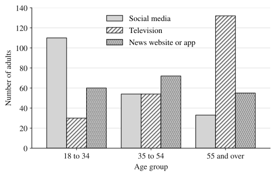
This graph is good for reading off individual counts, and the pattern within each cluster is easy to see. Its weakness is the one from the table: when groups differ in size, taller bars can just mean a bigger group. Comparing the 35 to 54 social-media bar (54) with the 55-and-over social-media bar (33) by height alone mixes up "more people in the group" with "a larger share of the group."
Segmented bar chart
A segmented bar chart (or stacked bar chart) gives each group one bar of height 1 (or 100%), divided into segments whose heights are the proportions within that group. It is the row-proportion table drawn as a picture.
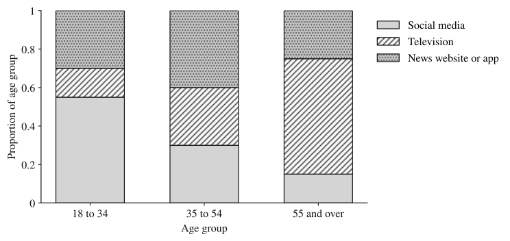
Because every bar has the same height, group size no longer distorts the picture, and you compare segment heights directly. The social-media segment shrinks from 0.55 to 0.30 to 0.15 as age increases, while the television segment grows from 0.15 to 0.30 to 0.60. The price is that the counts and the group sizes are gone: a bar for 20 people looks as solid as a bar for 2,000.
Mosaic plot
A mosaic plot is a segmented bar chart whose bar widths are proportional to the group sizes. Heights still show the proportions within each group, so the area of each rectangle is proportional to the count in that cell.
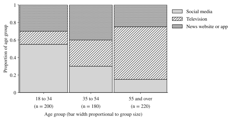
The mosaic plot shows both things at once: the 55-and-over group is the largest of the three (220 of 600), and its television rectangle is the largest single rectangle, which matches the largest count in the table, 132.
Association: when one variable's distribution changes with the other
Two categorical variables are associated if knowing an individual's category for one variable changes what you'd expect for the other. In table terms, the distribution of one variable is different across the categories of the other. In a segmented bar chart or mosaic plot, association looks like segment heights that change from bar to bar. No association looks like bars that are divided identically: every group splits across the categories in the same proportions.
The poll shows a clear association between age group and main news source. The share using social media falls from 0.55 to 0.15 across the age groups and the share using television rises from 0.15 to 0.60; if age and news source were unrelated, all three bars would split the same way.
Three points make a claim of association precise:
- Either direction works. You could instead split by news source and show the age distribution within each source. If the variables are associated one way, they are associated the other way too. Pick the direction that matches the question: compute proportions within the categories of the variable that defines the groups being compared. When one variable may explain or influence the other (the explanatory variable), those groups are its categories, and you compare the distribution of the other variable (the response variable, the outcome being explained) across them: here, news source within each age group.
- Sample data never match perfectly. Even if two variables were unrelated in the whole population, a sample would show bars that differ slightly by chance. Small differences are weak evidence; large ones, like 0.55 against 0.15, are strong. Topics 3.14 and 3.15 build a test (chi-square) for deciding how big a difference has to be.
- Association is not causation. These are survey data, not an experiment, so the graph shows that age and news source go together, not that getting older makes people switch to television. Habits formed when a person was young, before social media existed, could explain the pattern just as well.
Worked examples
A town has two public pools. One Saturday, staff recorded whether each visitor bought something at the snack bar. At Lakeside Pool, 90 of 300 visitors bought a snack. At Hill Pool, 48 of 120 visitors did. A council member says, "Lakeside visitors are more likely to buy snacks; 90 is almost twice 48." Make a two-way table and evaluate the claim.
Show solution
| Pool | Bought a snack | Did not | Total |
|---|---|---|---|
| Lakeside | 90 | 210 | 300 |
| Hill | 48 | 72 | 120 |
| Total | 138 | 282 | 420 |
"More likely" is a statement about proportions, so compare each pool's share. Lakeside: . Hill: .
The claim is not supported. On that Saturday, 40% of Hill Pool visitors bought a snack compared with 30% of Lakeside visitors, so a Hill visitor was more likely to buy one. Lakeside sold more snacks because it had 2.5 times as many visitors. A segmented bar chart would show this at a glance: Hill's "bought" segment (0.40) sits higher than Lakeside's (0.30).
A hospital surveys 400 staff about how they usually get to work. Of the 250 day-shift staff, 150 drive, 75 take the bus and 25 bike. Of the 150 night-shift staff, 90 drive, 45 take the bus and 15 bike. Describe the segmented bar chart with one bar per shift, and decide whether shift and commuting method are associated.
Show solution
Divide each shift's counts by that shift's total. Day: drive, bus, bike. Night: , , .
The two bars are divided identically: a 0.60 "drive" segment, a 0.30 "bus" segment and a 0.10 "bike" segment. Knowing someone's shift tells you nothing about how they commute, so shift and commuting method are not associated for these 400 staff.
Check the other direction to see that it agrees. Of the 240 drivers, work days; of the 120 bus riders, ; of the 40 bikers, . Every commuting group has the same day-shift share, which is also the overall share, . No association in one direction means none in the other.
A veterinary clinic surveyed 480 dog owners about their dog's size and whether they walk the dog at least twice a day.
| Dog size | Walks at least twice a day | Does not | Total |
|---|---|---|---|
| Small | 91 | 169 | 260 |
| Medium | 77 | 63 | 140 |
| Large | 60 | 20 | 80 |
| Total | 228 | 252 | 480 |
(a) A staff member makes a side-by-side bar chart of the counts and says, "Small-dog owners walk their dogs most, because their 'walks twice a day' bar is the tallest." Explain why this reasoning is flawed.
(b) Describe a segmented bar chart that compares walking habits across dog sizes, giving the height of each segment.
(c) Do these data suggest an association between dog size and walking at least twice a day? Justify your answer using your graph.
Show solution
(a) The tallest bar reflects the size of the group, not the habit. The 91 small-dog owners who walk twice a day come from a group of 260, more than three times as many owners as the large-dog group (80). Comparing counts from groups of different sizes can't say which group is more likely to walk; that takes the proportion within each group.
(b) One bar per dog size, each of height 1. The "walks at least twice a day" segment has height for small dogs, for medium dogs, and for large dogs. The "does not" segment fills the rest of each bar: 0.65, 0.45 and 0.25.
(c) Yes. The proportion of owners who walk their dog at least twice a day rises from 0.35 for small dogs to 0.55 for medium dogs to 0.75 for large dogs. The segments differ substantially from bar to bar, so in this sample, owners of larger dogs were more likely to walk their dog at least twice a day, which suggests an association between dog size and walking frequency.
Why these moves: part (a) earns credit by naming the specific problem (unequal group sizes) and the fix (proportions within groups). Parts (b) and (c) compute the proportions within each dog size, because dog size defines the groups being compared, and the answer to (c) quotes all three proportions, states the direction, and stays in context. It says "suggests an association," not "bigger dogs cause more walking": owners chose their dogs, so this is an observational survey.
Where students lose points
Check yourself
Question 1
A library records whether each borrower checked out fiction or nonfiction, for adult and teen borrowers. Of 400 adults, 240 checked out fiction; of 150 teens, 105 checked out fiction. Which statement is supported by the data?
- A
Adults were more likely to check out fiction, because 240 is more than 105.
- B
Teens were more likely to check out fiction: 70% of teens did, compared with 60% of adults.
- C
Borrower age and book type are not associated, because most borrowers in both groups chose fiction.
- D
Adults were more likely to check out fiction: 240 of the 345 fiction borrowers, about 70%, were adults.
Show answer
B
Likelihood within a group is the group's own proportion: for teens and for adults. Choice A compares counts from groups of different sizes. Choice C misses that 0.70 and 0.60 differ, and both groups having a majority does not mean the distributions match. Choice D divides by the fiction total (), which describes who the fiction borrowers were, not how likely each age group was to borrow fiction; adults dominate that group only because there are more adult borrowers.
- A
Question 2
Two segmented bar charts each compare three groups. In chart P, the bars are divided into segments of the same heights for all three groups. In chart Q, the bottom segment has heights 0.20, 0.45 and 0.70. Which chart shows an association between the two variables, and why?
Show answer
Chart Q. Its segment heights change from group to group, so the distribution of the second variable differs across the groups. In chart P every group splits the same way, so knowing the group tells you nothing about the other variable.
Association between categorical variables means the conditional distributions differ across categories. Identical segmented bars mean identical distributions, which is no association.
Question 3
A mosaic plot shows two bars. Bar 1 is three times as wide as bar 2, and the top segment of each bar has height 0.5. Which is true?
- A
The two groups have the same number of individuals in the top category.
- B
Group 2 has a larger proportion in the top category than group 1.
- C
Group 1 has three times as many individuals in the top category as group 2.
- D
The plot cannot show group sizes, so nothing can be said about counts.
Show answer
C
In a mosaic plot, heights are proportions within each group and widths are proportional to group sizes, so areas are proportional to counts. Both top rectangles have height 0.5, and the first is three times as wide, so it holds three times as many individuals. Choice D describes a segmented bar chart, not a mosaic plot.
- A
Question 4
A student surveys 90 ninth graders and 60 twelfth graders about whether they eat breakfast on school days. 54 ninth graders and 36 twelfth graders say yes. The student writes, "Ninth graders are more likely to eat breakfast." Is the claim supported? Justify.
Show answer
No. The proportion who eat breakfast is for ninth graders and for twelfth graders. The two grades have the same proportion, so these data give no evidence that ninth graders are more likely to eat breakfast; grade and eating breakfast show no association in this sample.
The larger count (54 against 36) only reflects that more ninth graders were surveyed. Comparing proportions within each grade shows identical distributions.