A food truck knows from months of receipts that about 30% of its customers order the daily special. The owner wants to know how often at least 3 of the first 5 customers will order it, because that is when the special runs out before the lunch rush. You could wait and watch hundreds of mornings. Or you can imitate the mornings with random numbers, thousands of times in a few seconds, and count how often the special runs out. That imitation is a simulation, and the fraction of times the event happens is an estimate of its probability.
Random processes, outcomes and events
A random process is a repeatable situation whose result is decided by chance: you know what results are possible, but not which one you'll get on a given try. A customer deciding what to order is one; so are rolling a die, dealing a card, or picking 4 employees at random from a list. One repetition of the process is a trial.
An outcome is the result of one trial. If one trial is "the next 5 customers order," an outcome is a full record of what happened, such as S N N S N (special, not, not, special, not).
An event is a collection of outcomes, usually named with a capital letter. The event = "at least 3 of the 5 order the special" contains every outcome with three or more S's: S S S N N, N S S S N, S S S S S, and many more. An event happens on a trial if the outcome of that trial is one of the outcomes in the event.
The distinction matters when you design a simulation: you simulate outcomes, then check each one against the event.
Probability as long-run relative frequency
The probability of an event is the proportion of times it would happen if the random process were repeated a very large number of times. That is a definition, not a formula: "the probability of rolling a 6 is " means that in a huge number of rolls, about one roll in six is a 6.
You will never see an infinite number of trials, but the relative frequency you observe in a real set of trials (the count of times the event happened, divided by the number of trials) is an estimate of the probability. The food truck's "about 30%" is exactly this: an estimate from many past customers.
How good is the estimate? The law of large numbers answers that: when trials are independent (one trial's result doesn't change the chances on another), the relative frequency of an event settles down to a single value, the probability, as the number of trials grows. The graph below follows the proportion of sixes in 1,000 simulated rolls of a fair die.
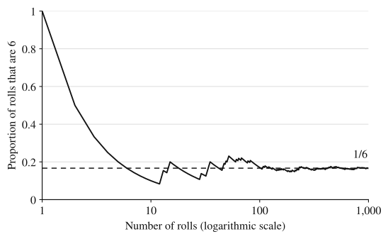
Early on, the relative frequency jumps around wildly: one 6 in the first roll makes it 1, and one 6 in the first 10 rolls makes it 0.1. Each new roll changes a proportion based on few rolls a lot and a proportion based on many rolls very little, which is why the line flattens out. After 1,000 rolls, 166 sixes give 0.166, very close to .
Read the law carefully. It describes the long run only. It does not say that after a string of non-sixes, a 6 is "due": the die has no memory, and each roll has the same chance. The proportion gets closer to because the early streaks get swamped by a growing number of later rolls, not because later rolls compensate for them.
Designing and running a simulation
A simulation replaces the real random process with a chance device (random digits, a random number generator, cards, coins) set up so that each simulated outcome has the same probability as the real one. On the exam, a description has to be complete enough that someone else could carry it out and get comparable results. That takes four parts.
- Assign values to outcomes so the probabilities match. For the food truck, each customer orders the special with probability 0.3. Using random digits 0 to 9, let 0, 1, 2 mean "orders the special" and 3 to 9 mean "does not." Three of the ten equally likely digits gives probability 0.3.
- Describe one trial and what to record. One trial is 5 consecutive digits, one per customer. Record how many of the 5 digits are 0, 1 or 2.
- Repeat many times. Do many trials, keeping track of the count of trials and the count of trials where the event happened.
- Estimate. The estimated probability is the number of trials where the event happened divided by the total number of trials.
Here are 40 digits from a random number table, split into 8 trials of 5 digits:
Count the 0s, 1s and 2s in each group: 2, 1, 3, 1, 1, 1, 3, 2. Trials 3 and 7 have at least 3 specials, so this run of 8 trials estimates the probability as .
Eight trials is far too few to trust; the law of large numbers says the estimate is only reliable with many trials. A computer running the same design for 500 trials gave these results:
| Specials ordered (of 5) | 0 | 1 | 2 | 3 | 4 | 5 |
|---|---|---|---|---|---|---|
| Number of trials | 91 | 184 | 150 | 60 | 15 | 0 |
At least 3 specials happened in of 500 trials, so the estimate is . The special runs out early on roughly 15% of mornings, about one weekday in seven. (Topic 2.10 computes this probability exactly; it is about 0.163, so the simulation landed close.)
Three design details need care:
- Probabilities that don't fit single digits. For a probability of 0.15, use pairs of digits: 00 to 14 for the event, 15 to 99 for not. For 0.25, you can use 0 and 1 for the event, 2 to 7 for not, and skip 8 and 9, which leaves 8 equally likely digits, 2 of them assigned to the event.
- Sampling without replacement. When the real process can't pick the same individual twice (choosing 4 different people), label the individuals, and skip any label that has already been chosen in the current trial. Also skip labels that match no one (00, or 13 to 99 if there are 12 people).
- Random number generators. On a calculator, randInt(1, 12) gives a random whole number from 1 to 12 with equal chances. The same rules apply: say what the numbers stand for, what one trial is, and whether repeats are skipped.
Worked examples
On a commuter flight, 15% of ticketed passengers don't show up. A family of 4 has tickets. Design a simulation to estimate the probability that at least one of the 4 doesn't show up (assume the passengers act independently), and carry out 5 trials with these random digits:
Show solution
Design. Read the digits in pairs, 00 to 99, each pair equally likely. Pairs 00 to 14 (15 of the 100) mean the passenger does not show up; pairs 15 to 99 mean the passenger shows up. One trial is 4 pairs, one per family member. Record whether at least one of the 4 pairs is between 00 and 14. Repeat for many trials; the estimate is the fraction of trials with at least one no-show.
Single digits won't work here: 15% is not a whole number of tenths, so two-digit pairs are needed to give the event probability exactly 0.15.
Trials (each group of 8 digits is 4 pairs):
- 28 03 78 90: 03 is a no-show. Event happens.
- 65 63 03 71: 03. Event happens.
- 36 71 37 28: no pair from 00 to 14. Event does not happen.
- 23 76 02 79: 02. Event happens.
- 56 94 03 84: 03. Event happens.
Estimate: . Five trials is far too few for a trustworthy estimate (topic 2.7's rules give the true value, about 0.478), which is why a real simulation runs hundreds or thousands of trials.
A student guesses on a 10-question true-false quiz, so each answer is right with probability 0.5. A computer simulated 1,000 such quizzes by flipping a virtual coin for each question (heads means correct) and recorded the number correct:
| Number correct | 0 | 1 | 2 | 3 | 4 | 5 | 6 | 7 | 8 | 9 | 10 |
|---|---|---|---|---|---|---|---|---|---|---|---|
| Number of quizzes | 0 | 10 | 48 | 111 | 197 | 272 | 197 | 111 | 45 | 6 | 3 |
(a) Estimate the probability that a guesser gets at least 8 right.
(b) A classmate says that if the computer ran 100,000 quizzes instead, the estimate would be exactly right. Is the classmate correct?
Show solution
(a) Quizzes with at least 8 correct: . The estimate is . A student who guesses on every question would get 8 or more right on about 5.4% of quizzes.
(b) No. The law of large numbers says the relative frequency from 100,000 quizzes would very likely be closer to the true probability than one from 1,000 quizzes, because the estimate settles down as the number of trials grows. It does not promise the estimate will equal the probability exactly; any finite number of trials leaves some chance variation.
Why these moves: in (a), "at least 8" means 8, 9 or 10, so you add three cells and divide by the total number of trials, 1,000. In (b), the answer turns on the difference between "closer and closer" and "exactly."
A restaurant has 12 employees: 5 part-time and 7 full-time. The manager says she picked 4 employees at random to work on a holiday, and all 4 chosen were part-time. The full-time staff are suspicious.
(a) Describe how to use a random number generator to carry out one trial of a simulation of the manager's random selection, recording whether all 4 selected employees are part-time.
(b) Here are the random integers from 1 to 12 produced for three trials. Carry out the three trials.
Trial 1: 2, 2, 10, 6, 8. Trial 2: 8, 9, 1, 6. Trial 3: 2, 5, 12, 7.
(c) In 200 trials of this simulation, all 4 selected employees were part-time in 2 trials. Estimate the probability that a random selection picks 4 part-time employees, and explain what this suggests about the manager's claim.
Show solution
(a) Label the part-time employees 1 to 5 and the full-time employees 6 to 12. Use randInt(1, 12) to generate random integers, skipping any number already chosen in this trial, until 4 different employees are selected. Record whether all 4 labels are from 1 to 5.
(b) Trial 1: the second 2 is a repeat, so skip it. The selected employees are 2, 10, 6, 8: one part-time, so not all part-time. Trial 2: 8, 9, 1, 6: one part-time, not all. Trial 3: 2, 5, 12, 7: two part-time, not all. In none of the three trials were all 4 selected employees part-time.
(c) The estimated probability is . If the manager truly picked 4 employees at random, all 4 would be part-time only about 1% of the time. An outcome that rare under random selection gives the full-time staff good reason to doubt that the selection was random.
Why these moves: in (a), repeats must be skipped because the same employee can't be chosen twice; a design that allows repeats simulates the wrong process and loses credit. Labeling 1 to 5 as part-time keeps the probabilities right, since each of the 12 employees is equally likely. In (c), the estimate comes from the simulation's counts, and the conclusion compares how often the observed result happens by chance alone. Later topics (3.6 onward) make this reasoning formal as a p-value.
Where students lose points
Check yourself
Question 1
A spinner lands on red with probability 0.4. Which assignment of random digits 0 to 9 correctly simulates one spin?
- A
0 to 4 is red, 5 to 9 is not red.
- B
0 to 3 is red, 4 to 9 is not red.
- C
1 to 4 is red, 5 to 9 is not red, and 0 is skipped.
- D
Read pairs of digits: 00 to 40 is red, 41 to 99 is not red.
Show answer
B
Four of the ten equally likely digits (0, 1, 2, 3) give probability . Choice A uses five digits, probability 0.5. Choice C leaves nine usable digits, so red has probability . Choice D includes 00 through 40, which is 41 pairs, probability 0.41.
- A
Question 2
You toss three coins and record the result of each, such as HTH. Is "exactly two heads" an outcome or an event? List what it contains.
Show answer
An event. It is the collection of outcomes HHT, HTH and THH.
An outcome is the full result of one trial (a specific sequence of three tosses). "Exactly two heads" is satisfied by three different sequences, so it is a set of outcomes, which is an event.
Question 3
A fair coin lands heads on 7 of its first 10 flips. It is then flipped 1,000 more times. Which statement is correct?
- A
The next 1,000 flips will include more tails than heads, to balance out the early heads.
- B
The probability of heads on the 11th flip is less than 0.5.
- C
The proportion of heads in all 1,010 flips will very likely be closer to 0.5 than 0.7 is.
- D
The number of heads in all 1,010 flips will be exactly 505.
Show answer
C
By the law of large numbers, the relative frequency settles near 0.5 as flips accumulate; the 7 early heads are swamped by 1,000 later flips, not cancelled. Choices A and B are the gambler's fallacy: independent flips have no memory, so each still has probability 0.5. Choice D claims an exact count, which no finite number of trials guarantees.
- A
Question 4
A simulation of a hockey team's season ran 250 times. In 85 of the simulated seasons, the team made the playoffs. Estimate the probability that the team makes the playoffs, and say what would make the estimate more reliable.
Show answer
. The team makes the playoffs in about 34% of simulated seasons. Running many more simulated seasons would make the estimate more reliable, because the relative frequency settles closer to the true probability as the number of trials grows.
The estimate is the number of trials in which the event happened divided by the total number of trials. The law of large numbers is the reason more trials help.