A food truck owner can't know how many drinks the next customer will order, but over thousands of orders a pattern is steady: 30% of orders have no drink, 45% have one, 15% have two, and 10% have three. A list like that, every possible number paired with its probability, is a probability distribution, and it's the object the rest of Unit 2 works with.
Random variables
A random variable is a numerical value determined by the outcome of a random process. Before the process runs, you don't know its value; afterward, the outcome fixes it. Random variables get capital letters, like , and a particular value gets the lowercase letter, like . So "" is the event that the random variable comes out to 2, and is its probability.
The definition has two parts that matter. The value must be a number: "the color of the next car" comes from a random process but isn't a random variable, while "the number of red cars among the next 10" is. And the number must come from chance: the number of days in March is always 31, so it isn't random.
A discrete random variable has values you can list with gaps between them, usually counts: the number of drinks in an order, the number of heads in 5 flips, the number of defective chips in a box. A random variable that can take any value in an interval, like the time until the next customer arrives, is continuous; topic 2.11 handles that kind. This topic is about discrete random variables.
Probability distributions
The probability distribution of a discrete random variable gives the probability of each of its possible values. Let = the number of drinks in a randomly selected order from the food truck:
| 0 | 1 | 2 | 3 | |
|---|---|---|---|---|
| 0.30 | 0.45 | 0.15 | 0.10 |
Two requirements make a table like this a valid distribution, and both come straight from topic 2.4:
Here , so the table is valid. The second requirement also lets you find one missing probability: if a table left out , it would have to be .
To find the probability of an event about , add the probabilities of the values in it, because the values are mutually exclusive. "At least two drinks" is :
With a discrete variable, the inequality sign changes the answer. leaves out the value 2, so it's only .
Three ways to show a distribution
A table, like the one above, lists each value and its probability.
A graph, usually a probability histogram, puts the values on the horizontal axis and draws a bar over each one whose height is its probability.
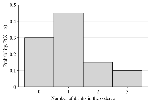
Shape, center and spread are read from it the same way as for a histogram of data (topic 1.6): this distribution peaks at 1 drink and is skewed right, with a tail toward 3.
A function gives the probability as a formula in . You'll see one in the next section.
Building a distribution from probability rules
When the random process is simple enough to list its outcomes, you can work the distribution out exactly. Roll two fair four-sided dice (faces 1 to 4) and let = the larger of the two numbers (if they match, that number). There are equally likely outcomes. Sort them by the value of :
- : only (1, 1). Probability .
- : (1, 2), (2, 1), (2, 2). Probability .
- : (1, 3), (2, 3), (3, 3), (3, 1), (3, 2). Probability .
- : the 7 outcomes with at least one 4. Probability .
The probabilities sum to . The pattern has a reason: means both dice are at most , which happens in outcomes, so exactly accounts for outcomes. That gives the distribution as a function:
The steps are always the same: list the sample space, find the value of for each outcome, and add the probabilities of the outcomes that give each value. When outcomes aren't equally likely, use the multiplication and addition rules from topics 2.6 and 2.7 to get each probability.
Estimating a distribution by simulation
Some processes are tedious to work out exactly. A simulation (topic 2.3) estimates the distribution instead: run the process many times with random numbers, record the value of in each trial, and use the relative frequency of each value as its estimated probability. More trials give estimates that tend to be closer to the true probabilities.
Cumulative distributions
A cumulative probability distribution gives, for each value , the probability that is less than or equal to : . Build it by keeping a running total down the table. For the food truck:
| 0 | 1 | 2 | 3 | |
|---|---|---|---|---|
| 0.30 | 0.45 | 0.15 | 0.10 | |
| 0.30 | 0.75 | 0.90 | 1.00 |
The cumulative column never decreases and ends at exactly 1, because every value of is at most the largest one. It answers "at most" questions in one look: , so three quarters of orders have at most one drink. With the complement rule it answers "more than" questions too, , and differences of cumulative values give ranges: .
For the dice maximum, the cumulative distribution is also a function: for , which is the count from before.
Worked examples
A hotel finds that the number of nights a randomly selected guest stays has this distribution.
| 1 | 2 | 3 | 4 | 5 | |
|---|---|---|---|---|---|
| 0.25 | 0.35 | 0.12 | 0.08 |
(a) Find . (b) Find the probability a guest stays at least 3 nights. (c) Find .
Show solution
(a) The probabilities must add to 1: , so and .
(b) "At least 3" includes 3: .
(c) The values with are 2 and 3 (4 is excluded by the strict sign): .
A cereal brand puts one of three toys in each box, each equally likely, independently from box to box. A family buys 4 boxes. Let = the number of different toys they get. A student simulates this 200 times: in each trial, a calculator generates 4 random integers from 1 to 3 (one per box, the integer naming the toy), and the student records how many different integers appear. The results:
| Different toys | 1 | 2 | 3 |
|---|---|---|---|
| Number of trials | 7 | 105 | 88 |
Estimate the probability distribution of , and estimate the probability that the family gets all three toys.
Show solution
Divide each count by the 200 trials:
| 1 | 2 | 3 | |
|---|---|---|---|
| Estimated | 0.035 | 0.525 | 0.440 |
The estimates add to , as they must. The estimated probability of getting all three toys is .
Each trial matches the real process: 4 boxes, each with an equally likely toy from 3, chosen independently. That's what makes the relative frequencies estimates of the true probabilities. Counting outcomes exactly gives , so 200 trials came close. A different 200 trials would give somewhat different estimates.
A student applies to three summer programs. The probabilities of acceptance are 0.6 for the first, 0.4 for the second, and 0.2 for the third, and the decisions are independent. Let = the number of programs that accept the student.
(a) Construct the probability distribution of .
(b) Construct the cumulative probability distribution of .
(c) Find the probability that the student is accepted to at least one program.
Show solution
(a) can be 0, 1, 2 or 3. The rejection probabilities are , and . Because the decisions are independent, the probability of any particular combination is a product (topic 2.7), and the combinations giving the same are mutually exclusive, so their probabilities add. Each product below lists the first, second and third program in that order.
For , the three terms are accepted by only the first, only the second, only the third. For , they are rejected by only the third, only the second, only the first.
| 0 | 1 | 2 | 3 | |
|---|---|---|---|---|
| 0.192 | 0.464 | 0.296 | 0.048 |
Check: .
(b) Running totals:
| 0 | 1 | 2 | 3 | |
|---|---|---|---|---|
| 0.192 | 0.656 | 0.952 | 1.000 |
(c) . The probability that the student is accepted to at least one of the three summer programs is 0.808.
Why these moves: listing each combination with its product shows the grader exactly where every probability comes from, and the sum-to-1 check catches a missed combination. Part (c) uses the complement because "at least one" is three values but "none" is one. This is not a binomial setting (topic 2.10), because the three acceptance probabilities differ.
Where students lose points
Check yourself
Question 1
Which of the following is a discrete random variable?
- A
The color of a randomly selected car in a parking lot
- B
The number of siblings a randomly selected student has
- C
The time a randomly selected runner takes to finish a 5-kilometer race
- D
The name of the team that wins a randomly chosen game
Show answer
B
A number of siblings is a numerical outcome of a random selection, and its values (0, 1, 2, ...) can be listed with gaps between them. Choice C is a random variable too, but time can take any value in an interval, so it is continuous; A and D are not numerical at all.
- A
Question 2
Which table gives a valid probability distribution for a random variable with values 0, 1, 2, 3?
- A
- B
- C
- D
(no probability listed for 3)
Show answer
C
C's probabilities are each between 0 and 1 and add to exactly 1. A adds to 1.1; B adds to 1 but includes a negative probability, which is impossible; D leaves out a value and adds to only 0.75.
- A
Question 3
The cumulative distribution of a random variable is , , , . Find and .
Show answer
and .
A single value's probability is the jump in the cumulative distribution at that value. "At least 2" is the complement of "at most 1," whose probability is the cumulative value at 1.
Question 4
A random variable has for . Show that this is a valid distribution and find .
Show answer
Each is between 0 and 1, and . .
A function is a valid distribution under the same two requirements as a table. Adding the probabilities of the values 4 and 5 gives the event "at least 4."