Graphical Representations for One Categorical Variable

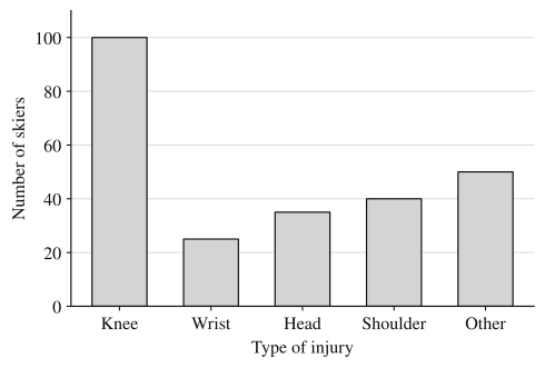
A ski resort's clinic recorded the type of injury for each of the 250 skiers it treated last season: 100 knee injuries, 25 wrist, 35 head, 40 shoulder and 50 other. Topic 1.3 put counts like these in a table. A graph shows the same information at a glance, so that the biggest category, and how much bigger it is, jump out before anyone reads a number. Two graphs do this for a categorical variable: the bar chart and the pie chart.

Bar charts

A bar chart (or bar graph) has one bar for each category. The bar's height (or its length, if the bars run sideways) is the category's frequency or relative frequency.

To build one:

1. Put the categories along one axis and label it with the variable's name.
2. Put a numerical scale on the other axis, starting at 0, labeled "Frequency" (or what was counted) or "Relative frequency."
3. Draw one bar per category, all the same width, with equal gaps between them, each reaching its category's value.

The gaps matter. They show that the categories are separate groups, not intervals on a number line, which is what a histogram's touching bars mean (topic 1.5). The order of the bars is a choice: for categories with no natural order, sorting from tallest to shortest makes comparisons easy; for ordered categories (Never, Sometimes, Often), keep their order.

A frequency bar chart and a relative frequency bar chart of the same data have exactly the same shape. Dividing every count by 250 rescales the axis and leaves every bar's height relative to the others unchanged. The difference only matters when two groups are compared, below.

Pie charts

A pie chart shows a whole divided into parts. Each category gets a slice, and the slice's share of the circle equals the category's relative frequency. Since the angles around the center add to $360°$, a category with relative frequency $r$ gets a slice with angle $r \times 360°$. The knee slice is $0.40 \times 360° = 144°$; the wrist slice is $0.10 \times 360° = 36°$.

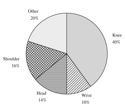
Because the slices fill the circle, they add to 1 (100%) of it, and that's the condition for using one: each unit must fall in exactly one category, and the categories must cover everyone. Two situations break it:

• Units in more than one category. A survey asking "Which streaming services do you use? Check all that apply" lets one person count for several services, so the percentages add to more than 100%. There is no whole for the slices to divide. Use a bar chart, with each bar showing the percentage of respondents who use that service.
• A missing category. If a report gives percentages for Knee, Wrist and Head only (64% together), a pie with only those three slices would make each look bigger than it is. Add the remaining category ("Other," 36%) or use a bar chart.

Pie charts are good at one comparison: a part against the whole ("knee injuries were 40% of the total, a bit less than half"). Bar charts are better for comparing categories with each other, because the eye judges heights from a common baseline more accurately than angles. In the pie above, the Head (14%) and Shoulder (16%) slices are hard to rank by eye; in the bar chart it's obvious.

Using a graph to back a claim

A claim about a categorical variable is supported by a graph when you can read off the specific values that make it true and say them in context. "Knee injuries were the most common type among the clinic's injured skiers: 100 of 250, or 40%" uses the graph. "The knee bar is biggest" describes the picture without saying what it means.

Read the scale before you read the bars. Here is the proportion of skiers with knee injuries next to the proportion of snowboarders with knee injuries (0.16, from the clinic's 150 injured snowboarders), with a vertical axis that starts at 0.15 instead of 0:

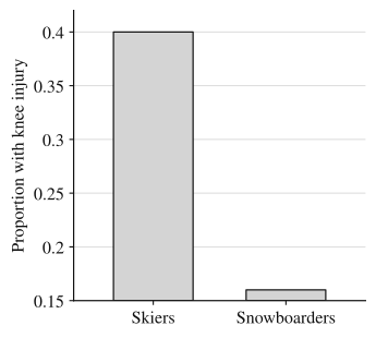
The skier bar looks about 25 times as tall as the snowboarder bar, because the visible parts are $0.40 - 0.15 = 0.25$ and $0.16 - 0.15 = 0.01$. The real ratio is $\frac{0.40}{0.16} = 2.5$. Bar heights only compare honestly when bars start at 0. When an axis doesn't, base your claim on the values, not the look.

Comparing groups

To compare two or more groups on the same categorical variable, graph each group's relative frequencies. The clinic also treated 150 snowboarders: 24 knee, 54 wrist, 21 head, 27 shoulder and 24 other injuries. Frequency bars would put 250 skiers against 150 snowboarders, and almost every skier bar would be taller just because there were more skiers. Dividing by each group's own total puts both on the same scale, and a side-by-side bar chart shows each category's bars next to each other:

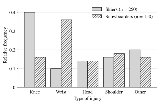
Two pie charts, one per group, also compare groups, since each pie is already in proportions. They make "what share of each group" easy to see but category-by-category differences harder; the side-by-side bar chart lines those up.

Worked examples

Where students lose points