A list of 30 daily high temperatures tells you very little until you can see where the values pile up and where they thin out. That pattern, which values occur and how often, is the variable's distribution. For a categorical variable, topic 1.4 showed it with bars in any order. A quantitative variable's values sit on a number line, so its graphs keep them in numerical order, smallest to largest, and that order is what lets you see clusters, gaps and extremes. Three graphs do the job: dotplots, stem-and-leaf plots and histograms.
Dotplots
A dotplot draws a number line for the variable and puts one dot above each observation's value. Equal (or nearly equal) values stack up in a column.
A youth soccer team scored these numbers of goals in its 22 games: three games with 0 goals, six with 1, seven with 2, three with 3, two with 4 and one with 6.
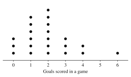
Every observation is its own dot, so you can recover the whole data set from the graph and count anything you need: the team scored 2 or more goals in of its 22 games. The empty spot at 5 matters too. The axis is a number line, so 5 gets its place even though no game had 5 goals, and the game with 6 goals stands apart from the rest. (Topic 1.6 gives the words for features like that.)
To build one: draw and label a number line covering the smallest to the largest value with an even scale, then place one dot per observation, stacking repeats evenly so that column heights compare honestly. The number line can also run vertically, with the dots lined up beside it instead of stacked above it. Dotplots work best for small data sets, up to a few dozen values; with hundreds of dots the stacks become unreadable.
Stem-and-leaf plots
A stem-and-leaf plot (stemplot) also keeps every value, but writes it with digits instead of dots. Each value is split into a stem (all but its last digit) and a leaf (its last digit, or the last digit you keep if you round first). Here are the lengths, in minutes, of the 15 episodes of a podcast's first season:
23, 31, 35, 38, 41, 42, 42, 44, 47, 49, 52, 55, 58, 61, 76
The stems are the tens digits, 2 through 7, written in a column from smallest to largest with a vertical line to their right. Each leaf goes beside its stem, in increasing order:
Key: minutes.
Turned on its side, a stemplot is a graph: the row of leaves is a bar whose length is the number of values in that stem's range. The 40s row is longest, so 40 to 49 minutes is the most common range, with 6 of the 15 episodes, and you can still read every exact value. Three rules keep it honest:
- Include a key. could mean 41 minutes, 4.1 hours or 410 people. Without the key the graph has no units and no scale.
- List every stem in the range, even if it has no leaves. If no episode had been in the 60s, the stem 6 would still appear, with nothing beside it, so the gap shows.
- Use one digit per leaf, and line the leaves up. Values with more digits than you need can be rounded or truncated first: 247 seconds could go on stem 24 with leaf 7 (key seconds), or be rounded to 250, counted in tens as 25, and placed on stem 2 with leaf 5 (key seconds). The key tells the reader which, and the rounded plot no longer shows the 7.
When almost all the values share two or three stems, the plot is too squashed to show anything. Split stems fix this by giving each stem two rows: leaves 0 to 4 on the first row and 5 to 9 on the second. Worked Example 3 below uses them.
Histograms
A histogram groups values into intervals of equal width, called bins (or classes), and draws a bar over each bin whose height is the number of observations in it (frequency) or the fraction of all observations in it (relative frequency). The bins sit along the number line in order and share their edges, so the bars touch. A gap between bars means an empty bin, which is information, just like the empty spot at 5 goals in the dotplot.
Building one takes two decisions and a rule.
- Where to start, and how wide to make the bins. Pick a convenient starting value at or below the minimum and a convenient width, such as 1, 2, 5 or 10 units, that gives roughly 5 to 15 bins. Every bin must have the same width.
- The boundary rule. A value exactly on an edge belongs to the bin it starts. With bins and , a 55 goes in the second. Each value lands in exactly one bin, so the frequencies add to .
- Frequency or relative frequency. A relative frequency histogram divides every bar's height by . Its bars have exactly the same shape; only the vertical scale changes. Relative frequency is the choice when you'll compare data sets of different sizes.
Most histograms put the bins on the horizontal axis with vertical bars, but you can also run the bins up the vertical axis with horizontal bars; the meaning is the same.
A histogram gives up the exact values, unless each bin is so narrow that it can hold only one possible value (bins 1 unit wide for whole-number data), in which case it is a dotplot drawn with bars. From the bar over 70 to 75 you know how many values are in that range but not what they are. That's the price of being able to show 30 or 30,000 values in the same tidy picture.
Bin width changes the picture
Here are the daily high temperatures for the 30 days of April in one city, in °F:
47, 50, 52, 53, 54, 54, 55, 56, 57, 57, 58, 59, 61, 62, 64, 65, 66, 67, 69, 70, 71, 71, 72, 73, 73, 74, 75, 76, 78, 81
These are two histograms of the same 30 values, one with bins 10 degrees wide and one with bins 5 degrees wide, both starting at 45.
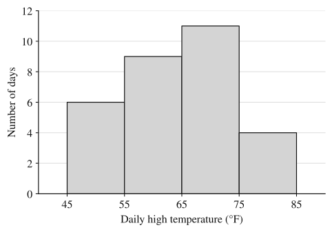
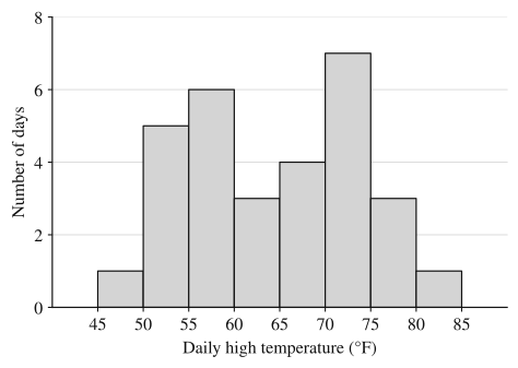
The wide bins show one hump. The narrow bins show two clusters, a cooler group of days in the 50s and a warmer group in the low 70s, with fewer days in between. Neither graph is wrong: both follow the rules, and the data are the same. Wide bins average over detail, so features narrower than a bin disappear. Bins that are too narrow have the opposite problem: with only 30 values and bins 1 degree wide, most bars would be 0, 1 or 2 tall and the picture would be noise. When you draw a histogram, try more than one width and pick the one that shows the pattern without the noise; when you read one, remember that a different bin choice might show something this one hides.
Worked examples
The ages of the 18 people in a community pottery class are:
33, 58, 19, 45, 64, 27, 52, 38, 22, 67, 41, 33, 58, 24, 46, 63, 55, 31
Make a stemplot, and find the percentage of the class aged 50 or older.
Show solution
The ages run from 19 to 67, so the stems are the tens digits 1 through 6. Place each leaf beside its stem, then put the leaves on each stem in order:
Key: years old.
Check the count: leaves, one per person. Both 33s and both 58s appear, once each as a separate leaf.
Ages 50 or older are the leaves on stems 5 and 6: people. , so about 38.9% of the class is 50 or older. The stemplot made this a count instead of a search through the list, and the exact ages are still there if you need them.
A consumer group ran 20 new phones of one model until their batteries died. Battery life, in hours:
9.4, 10.2, 11.8, 10.7, 12.3, 10.0, 11.1, 9.8, 10.5, 13.0, 11.4, 10.9, 12.0, 11.6, 10.3, 11.0, 12.7, 10.6, 11.2, 14.1
Make a frequency table and a relative frequency table using bins 1 hour wide starting at 9, and describe the histogram.
Show solution
The values run from 9.4 to 14.1, so bins of width 1 from 9 to 15 give six bins. Values on an edge (10.0, 11.0, 12.0, 13.0) go in the bin they start.
| Battery life (hours) | Frequency | Relative frequency |
|---|---|---|
| 2 | ||
| 7 | ||
| 6 | ||
| 3 | ||
| 1 | ||
| 1 | ||
| Total | 20 |
The histogram has "Battery life (hours)" on the horizontal axis marked 9 through 15, and six touching bars of heights 2, 7, 6, 3, 1 and 1 (or 0.10, 0.35, 0.30, 0.15, 0.05 and 0.05 on a relative frequency scale). The tallest bar is 10 to 11 hours, and the bars shrink steadily toward 15 hours. Note where 13.0 went: into , not . Putting it in both would make the total 21.
Use the 30 April high temperatures and the two histograms of them above.
(a) Construct a stemplot of the temperatures using split stems.
(b) Explain why the two histograms look different, and identify a feature of the distribution that the histogram with 5-degree bins shows and the one with 10-degree bins does not.
(c) Using only the histogram with 5-degree bins, find the proportion of April days with a high below 60°F. Can you use that histogram to find the highest temperature of the month? Explain.
Show solution
(a) Stems are the tens digits, each split into a row for leaves 0 to 4 and a row for leaves 5 to 9:
Key: °F. (The first row is the 45 to 49 half of stem 4 and the last is the 80 to 84 half of stem 8; their other halves are empty and could be listed with no leaves.)
(b) Both histograms show the same 30 temperatures; they differ only in bin width. Each 10-degree bin combines two 5-degree bins, so the counts 1 and 5 merge into 6, 6 and 3 into 9, 4 and 7 into 11, and 3 and 1 into 4. The 5-degree histogram shows two clusters of days, one with highs from 50 to 60°F and one from 70 to 75°F, separated by fewer days in the 60s. The 10-degree bins merge the dip at 60 to 65 with the cluster beside it, so that histogram shows a single peak at 65 to 75°F.
(c) Days below 60°F are the bins 45 to 50, 50 to 55 and 55 to 60: days, so the proportion is . Forty percent of the days in April had a high below 60°F. The highest temperature can't be found from the histogram: it shows only that one day's high was somewhere from 80 up to (but not including) 85°F. The stemplot in part (a), or the data list, shows it was 81°F.
Why these moves: (a) keeps both rules a grader checks (ordered leaves, a key). (b) names the cause (the bin width, not the data) and a specific feature with its values, in context. (c) adds bins that lie entirely below 60, which works only because 60 is a bin edge, and explains the limit of a histogram instead of guessing a value.
Where students lose points
Check yourself
Question 1
A data set of 40 whole numbers between 10 and 99 could be displayed in any of these ways. From which display could you always recover every exact value in the data set?
- A
A histogram with bins 5 units wide
- B
A relative frequency histogram with bins 2 units wide
- C
A stem-and-leaf plot with a key
- D
A bar chart of the number of values above and below the mean
Show answer
C
Each leaf in a stemplot, read with its stem and the key, is one exact value. A histogram shows only how many values fall in each bin, and a bin 2 or 5 units wide holds more than one possible whole number (the bin from 10 to 12 holds both 10 and 11), so it can't say which of them a value is. Bins 1 unit wide would work for whole numbers, since each bin would then hold a single possible value, but no choice offers that.
- A
Question 2
A stemplot of the weights of seven newborn lambs has three rows: stem 2 with leaves 5 and 8; stem 3 with leaves 0, 2, 2 and 7; and stem 4 with leaf 1. The key is kilograms. How many of the lambs weighed more than 3.0 kilograms?
Show answer
lambs (3.2, 3.2, 3.7 and 4.1 kg)
With the key, the weights are 2.5, 2.8, 3.0, 3.2, 3.2, 3.7 and 4.1 kg. The value 3.0 is not more than 3.0, so it doesn't count, and each repeated leaf is a separate lamb.
Question 3
A histogram of the ages of the members of a gym uses bins , , , and so on. In which bin does a member who is exactly 30 years old belong?
- A
- B
- C
Both bins, since 30 is on the edge of each
- D
Neither bin; the value is left out
Show answer
B
A value on an edge belongs to the bin it starts, here , as the inequality says. Counting it twice or leaving it out would make the frequencies add to something other than the number of members.
- A
Question 4
A relative frequency histogram of the commute times of 80 employees has four bars, of heights 0.10, 0.25, 0.40 and 0.25. How many employees are in the tallest bar's bin?
Show answer
employees
A relative frequency is a count divided by , so the count is . The heights add to , as they must when every employee is in exactly one bin.