Descriptions for One Quantitative Variable Distributions

A histogram of how long 60 callers waited on hold is a picture, and an exam question will ask you to put that picture into words. A complete description names four things: the shape of the distribution, where its center is, how much variability (spread) it has, and any unusual features such as outliers, gaps or clusters. Every one of them is stated about the variable in context, with its units, so that a reader who never sees the graph still knows what the data look like.

Shape: which way the tail runs, and how many peaks

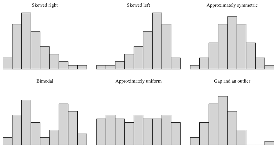
Skewness is named for the tail, not the peak. A distribution is skewed right (positively skewed) when the values trail off in a long tail toward the large numbers, so most of the data sit on the left and a few values stretch far to the right. It is skewed left (negatively skewed) when the long tail points toward the small numbers. It is approximately symmetric when you could fold the graph at its middle and the two halves would roughly match.

Skew usually has a cause you can name, and naming it is a good check on your reading of the graph. Times, prices and incomes are often skewed right because they can't go below 0 but have no fixed ceiling: most phone calls are short, and a few run for an hour. Scores on an easy quiz are often skewed left because they pile up against the maximum score and only a few students trail off toward low scores.

The second part of shape is the number of peaks. A distribution with one clear peak is unimodal. One with two distinct peaks is bimodal, and that is usually a sign that two different groups have been mixed in one data set: the heights of everyone at a school that includes both a kindergarten and a high school would show one peak for each age group. A distribution whose bars are all roughly the same height, with no peak standing out, is approximately uniform; the last digits of 500 randomly chosen phone numbers would look like this.

Real data are never perfectly symmetric or perfectly flat. Write "approximately symmetric" or "roughly uniform", and don't call a shape bimodal because one bar is slightly taller than its neighbor. A second peak has to stand out clearly, as it does in the bimodal panel above.

Center and spread, read from the graph

For a description, the center is a typical value: roughly where you would split the data into a lower half and an upper half. The spread says how far the values range, from the smallest to the largest. You can estimate both from a graph by counting. With 60 values in a histogram, the middle sits between the 30th and 31st values, so add bar heights from the left until you pass 30; the bar where that happens contains the center.

Topic 1.7 turns these into exact summary statistics (the mean, median, range, interquartile range and standard deviation). In a description, an approximate value with units is enough: "a typical caller waited about 3 minutes, and hold times ranged from 0 to about 20 minutes."

Unusual features: outliers, gaps and clusters

An outlier is a value that sits far below or far above the bulk of the data. On a graph you spot it as a bar or a dot standing off by itself. Topic 1.7 gives two numerical rules for deciding whether a value counts as an outlier; when you only have a graph, call it a "possible outlier" and give its value.

A gap is an interval of the number line where no observations fall even though there are data on both sides of it. Clusters are groups of values bunched together, usually with gaps between them. A gap is information: in the "gap and an outlier" panel, the empty classes are what make the lone bar on the right look unusual.

These features matter because they often point to something real. An outlier can be a recording error (a person's age entered as 340) or a genuine extreme (one customer who spent 40 minutes in a store). Clusters often mean the data come from different groups that behave differently, and that is worth saying in context.

Using a graph to support or refute a claim

A claim about the data ("most callers wait less than 5 minutes", "fewer than 10% of batteries fail before 6 hours") can be checked by counting from the graph. Add up the counts in the bars the claim is about, divide by the total, and compare the result with what the claim says.

Two things limit what a histogram can tell you. You know how many values fall in each class but not where inside the class they fall, so a claim that splits a class in the middle can't be checked exactly. And you must know which class gets a boundary value: in this lesson, a class like $[4, 6)$ includes 4 and excludes 6. A dotplot or stemplot shows every individual value, so counts from those graphs are exact.

Worked examples

Worked exampleExample 3: an exam-style description and claim

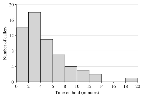
A phone company recorded the time each of 60 randomly selected callers spent on hold before reaching an agent. The histogram summarizes the times. Each class includes its left endpoint, so the first bar counts times from 0 up to (but not including) 2 minutes.

(a) Describe the distribution of hold times.

(b) The company's website says that three out of four callers reach an agent in under 6 minutes. Does the histogram support this claim? Justify your answer.

Show solution

(a) The distribution of hold times is unimodal and skewed right: most callers waited less than 6 minutes, with the tallest bar from 2 to 4 minutes, and a long tail stretches toward longer waits. The center is about 3 minutes: the first bar holds 14 callers and the first two hold 32, so the 30th and 31st hold times both fall in the 2-to-4-minute class. Hold times varied from 0 to about 20 minutes. There is a gap from 14 to 18 minutes, and the one caller who waited between 18 and 20 minutes is a possible outlier.

(b) Callers who waited under 6 minutes are those in the first three bars: $14 + 18 + 11 = 43$ callers. That is $\frac{43}{60} \approx 0.717$, or about 71.7% of the callers. Three out of four is 75%, so in this sample fewer than three out of four callers reached an agent in under 6 minutes. The histogram does not support the claim.

The justification is the comparison: a computed proportion (71.7%) set against the claimed one (75%). A bare "no" earns nothing, and so does "most callers waited under 6 minutes", which is true but doesn't address three out of four.

Where students lose points

On the exam

A free-response question that says "describe the distribution" wants shape, center, variability and unusual features, all in context. When it says "compare", Topic 1.9 adds the requirement to use comparative words ("greater than", "more variable"). For a claim, show the counts or the proportion you used and compare it with the claim's number before you state whether the graph supports it.