Graphical Representations of Summary Statistics for One Quantitative Variable

Five numbers from Topic 1.7 (the minimum, $Q_1$, the median, $Q_3$ and the maximum) cut a sorted data set into four pieces holding about a quarter of the values each. A boxplot draws those cuts on a number line, so you can see at a glance where the middle half of the data sits, which side is more stretched out, and which values are outliers.

The five-number summary and the boxplot

The five-number summary is the minimum, $Q_1$, the median, $Q_3$ and the maximum, in that order. A boxplot (box-and-whisker plot) is its picture:

• A box runs from $Q_1$ to $Q_3$, so it holds the middle 50% of the data, and its length is the IQR.
• A line inside the box marks the median.
• Whiskers run from the ends of the box outward. Without outliers, one goes from $Q_1$ down to the minimum and the other from $Q_3$ up to the maximum, so each whisker covers about 25% of the data.
• With outliers, each whisker stops at the most extreme value that is not an outlier, and every outlier is drawn as its own point (a dot or an asterisk). Outliers are found with the $1.5 \times \text{IQR}$ rule from Topic 1.7.

The four pieces (lower whisker, lower half of the box, upper half of the box, upper whisker) each hold about a quarter of the values, whatever their lengths. A long piece means those values are spread out, not that there are more of them. Pieces can also have zero length: if a quarter of the values all equal the minimum, then $Q_1$ equals the minimum and the lower whisker disappears.

Building a boxplot with outliers takes four steps: find the five-number summary, compute the fences $Q_1 - 1.5 \times \text{IQR}$ and $Q_3 + 1.5 \times \text{IQR}$, draw the box and median, then draw each whisker to the most extreme data value inside the fences and plot anything beyond them as a separate point. Always draw it on a number line with a scale and a label for the variable.

Reading shape from a boxplot

A boxplot shows skew through the lengths of its pieces. In a right-skewed distribution, the upper quarters are stretched: the median sits closer to $Q_1$ than to $Q_3$, the right whisker is longer than the left, and any outliers are usually on the high side. A left-skewed distribution is the mirror image. In a roughly symmetric distribution, the median is near the middle of the box and the two whiskers are about the same length.

What a boxplot can't show is anything inside a quarter. Gaps, clusters and the number of peaks are invisible: a bimodal data set with a hole in the middle and a single-peaked data set can have exactly the same five-number summary and therefore the same boxplot. A boxplot also doesn't show how many values there are. When those features matter, use a histogram, dotplot or stemplot.

Where the mean falls: mean versus median

The median only cares about the middle position, but the mean is the balance point of every value (Topic 1.7). In a skewed distribution the long tail holds values far from the center on one side, and the mean slides toward them to stay balanced. The median doesn't move with them.

The word "usually" is real. With lumpy, discrete data (such as counts with only a few possible values), a distribution can be skewed one way while the mean and median sit the other way or are equal. So the mean-median comparison is evidence about shape, not proof. When a question gives you only a mean and a median, say the shape is "likely" skewed right or left, and give the reason: the mean is pulled toward the tail.

Worked examples

Worked exampleExample 1: construct a boxplot with an outlier

The ages, in years, of 20 cars in a parking lot are

1, 2, 2, 3, 3, 4, 4, 5, 5, 5, 6, 6, 7, 7, 8, 9, 10, 11, 13, 24.

The mean age is 6.75 years. Construct a boxplot of the car ages, and explain what the mean and median suggest about the shape.

Show solution

Five-number summary. With $n = 20$, the median is the mean of the 10th and 11th values: $\frac{5 + 6}{2} = 5.5$ years. The lower half is the first 10 values, whose middle two are 3 and 4, so $Q_1 = 3.5$; the upper half is the last 10, whose middle two are 8 and 9, so $Q_3 = 8.5$. The minimum is 1 and the maximum is 24.

Fences. $\text{IQR} = 8.5 - 3.5 = 5$ years, and $1.5 \times 5 = 7.5$. The fences are $3.5 - 7.5 = -4$ and $8.5 + 7.5 = 16$ years. The 24-year-old car is above 16, so it is an outlier. Nothing is below $-4$.

Draw. The box runs from 3.5 to 8.5 with a line at 5.5. The left whisker goes to the minimum, 1. The right whisker stops at 13, the largest age that is not an outlier, and 24 is plotted as a separate point.

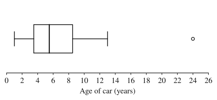
Shape. The mean (6.75 years) is greater than the median (5.5 years), and the boxplot agrees: the upper half of the box (5.5 to 8.5) is longer than the lower half (3.5 to 5.5), the right whisker is longer than the left, and the outlier is on the high side. The distribution of car ages is skewed right. The 24-year-old car pulls the mean up but not the median.

Worked exampleExample 2: reading a boxplot

The boxplot summarizes the one-way commute distances, in miles, of a company's 80 employees.

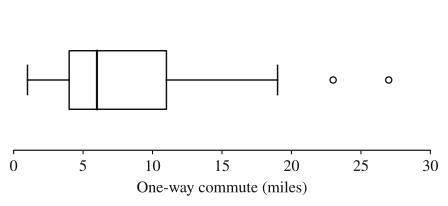
(a) About how many employees commute more than 11 miles? (b) Describe the shape, and predict whether the mean commute is greater or less than 6 miles.

Show solution

(a) 11 miles is $Q_3$, and about 25% of the values are above $Q_3$. So about $0.25 \times 80 = 20$ employees commute more than 11 miles. (Ties at exactly 11 make this approximate, which is why the answer says "about".)

(b) The upper half of the box, from 6 to 11 miles, is $11 - 6 = 5$ miles long, while the lower half is $6 - 4 = 2$ miles. The right whisker covers $19 - 11 = 8$ miles, the left only $4 - 1 = 3$ miles, and both outliers (23 and 27 miles) are high. Each of these pieces holds about a quarter of the employees, so the upper quarters are spread over much more distance: the distribution of commute distances is skewed right. A right skew pulls the mean toward the long tail, so the mean commute is likely greater than the median of 6 miles.

Worked exampleExample 3: from summary statistics to a boxplot (exam style)

A teacher reports these statistics for the final exam scores of 60 students:

$$\begin{array}{ccccccc} \bar{x} & s & \text{Min} & Q_1 & \text{Median} & Q_3 & \text{Max} \\ \hline 71.4 & 15.2 & 18 & 64 & 76 & 84 & 98 \end{array}$$

The lowest score that is not an outlier is 41. (a) Is there an outlier at either end? Justify. (b) Construct a boxplot of the scores. (c) Explain how the mean and median are consistent with the shape of the distribution.

Show solution

(a) $\text{IQR} = 84 - 64 = 20$ points and $1.5 \times 20 = 30$. The lower fence is $64 - 30 = 34$ and the upper fence is $84 + 30 = 114$. The minimum score of 18 is below 34, so 18 is a low outlier. The maximum, 98, is below 114, so there are no high outliers.

(b) Draw a box from 64 to 84 with a line at 76. The left whisker runs from 64 down to 41, the lowest score inside the fence, and 18 is plotted as a separate point. The right whisker runs from 84 to 98.

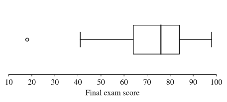
(c) The left whisker ($64 - 41 = 23$ points) is longer than the right ($98 - 84 = 14$ points), the lower half of the box ($76 - 64 = 12$) is longer than the upper half ($84 - 76 = 8$), and the outlier is on the low side, so the distribution of scores is skewed left. In a left-skewed distribution the low scores in the long tail pull the mean down, so the mean (71.4) is less than the median (76), as the data show.

Where students lose points

On the exam

A boxplot question can ask you to construct one (show the fences when there's an outlier and label the axis with the variable and units), to estimate a count or percentage from the quartiles, or to judge shape from the pieces. When summary statistics are given without a graph, the exam can ask you to compare the mean with the median, or the distances from the median to each quartile, and name the likely skew.