Comparisons of the Distributions for One Quantitative Variable

Do fish grow longer in one lake than another? Do people assemble furniture faster with video instructions than with a printed sheet? Questions like these compare the distribution of one quantitative variable across two or more groups, using the graphs and summary statistics of Topics 1.6 to 1.8 side by side.

A comparison uses comparative words

Comparing two distributions means comparing the same four features as in a description (shape, center, variability and unusual features), and stating how they differ. "Lake A's lengths have a median of 28.5 cm; Lake B's have a median of 22.5 cm" lists two facts. "The median length of the Lake A fish (28.5 cm) is greater than the median length of the Lake B fish (22.5 cm)" compares them. The second is what a comparison question asks for, and the exam scores it that way.

Each feature gets its own comparative statement:

• Shape: are both skewed the same way, or is one symmetric and the other skewed?
• Center: which group has the greater median (or mean)?
• Variability: which group is more spread out, by IQR, range or standard deviation?
• Unusual features: does one group have outliers, gaps or clusters that the other doesn't?

All of it is in context: name the variable, the groups and the units. Numerical summaries such as means, medians, standard deviations and IQRs can back up each statement, and when two measures disagree (a similar IQR but a much larger range, for instance) say what each one shows.

What each graph can and can't compare

To compare fairly, plot the groups on the same scale: one number line shared by parallel boxplots or stacked dotplots, or a back-to-back stemplot with one column of stems.

• Dotplots, stemplots and histograms show every feature: shape, center, variability, outliers, gaps and clusters. A back-to-back stemplot puts one group's leaves on the left of the stems and the other group's on the right, so the leaves on the left are read from right to left.
• Parallel boxplots compare centers (medians), variability (IQR and range), outliers and skew, and they make those comparisons quicker to read than any other display. They hide gaps, clusters and the number of peaks (Topic 1.8), and they don't show how many values are in each group.
• Histograms of groups with different sizes should use relative frequency (proportion of the group in each class) on the vertical axis. With counts, a class with 20 out of 200 values looks taller than one with 15 out of 30, even though it holds a much smaller share of its group.

Justifying a claim from a comparison

Many claims about groups can be checked with quartiles, because each quartile tells you a percentage. If the third quartile of group A is below the median of group B, then at least 75% of group A falls below a value that at least half of group B reaches or exceeds. That is strong evidence that group A's values tend to be lower. The reverse comparison works too: a box that lies entirely to one side of the other group's median says the same thing about the middle half of the data.

A claim based on centers alone can mislead when the spreads are large. Two groups with medians of 30 and 32 but IQRs of 20 overlap so much that most individuals in the "higher" group aren't higher than most individuals in the other. Before concluding that one group's values are larger, look at how much the distributions overlap.

z-scores: comparing positions across distributions

A sprinter's 100-meter time and a long jumper's distance can't be compared directly: they're in different units, and a "good" value means opposite things (low for the time, high for the distance). What you can compare is how unusual each value is within its own distribution. A standardized score, or z-score, turns a value into a count of standard deviations from its own distribution's mean, with a sign that says which side of the mean it is on.

The units cancel (minutes over minutes), so z-scores from different variables are on the same scale and can be compared. A larger $|z|$ means a value is farther from its own mean relative to that distribution's typical spread. Whether a positive or negative z-score is "better" depends on the variable: in a race, the time with the most negative z-score is the most impressive.

Rearranged, the formula turns a z-score back into a value: $x = \mu + z\sigma$. A value 1.5 standard deviations below a mean of 70 with $\sigma = 6$ is $70 - 1.5(6) = 61$.

Worked examples

Worked exampleExample 3: parallel boxplots and a claim (exam style)

A furniture company randomly assigned 60 volunteers to assemble the same bookshelf, 30 with printed instructions and 30 with video instructions, and recorded each assembly time in minutes.

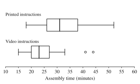
The means and standard deviations were: printed, $\bar{x} = 32.0$ and $s = 8.1$ minutes; video, $\bar{x} = 24.6$ and $s = 6.3$ minutes.

(a) Compare the distributions of assembly time for the two groups. (b) The company claims that most people using the video finish faster than a typical person using printed instructions. Do the boxplots support this claim? Justify your answer.

Show solution

(a) Center: the median assembly time with video instructions (23 minutes) is less than with printed instructions (31 minutes), and so is the mean (24.6 against 32.0 minutes).

Variability: times with printed instructions are more variable. Their IQR is $38 - 26 = 12$ minutes against $27 - 20 = 7$ minutes for video, their range is $52 - 18 = 34$ minutes against $44 - 15 = 29$ minutes, and their standard deviation is larger (8.1 against 6.3 minutes).

Shape: both distributions are slightly skewed right. In each, the upper part of the box and the upper whisker are longer than the lower ones, and the video group's outliers are on the high side.

Outliers: the video group has two high outliers, 41 and 44 minutes (beyond its upper fence of $27 + 1.5(7) = 37.5$ minutes); the printed group has none, since its fences are $26 - 18 = 8$ and $38 + 18 = 56$ minutes.

(b) Yes. The third quartile of the video times, 27 minutes, is below the median of the printed times, 31 minutes. So at least 75% of the video group finished in 27 minutes or less, faster than the typical (median) printed-instruction time of 31 minutes. Since 75% is a majority, the boxplots support the claim. Because the treatments were randomly assigned, a difference this large is evidence that the instructions caused it (Topic 1.10 explains why).

Where students lose points

On the exam

Comparison questions can come with parallel boxplots, side-by-side dotplots, back-to-back stemplots or a table of summary statistics. A complete answer compares every feature the question names, with numbers and comparative words, in context. A z-score question expects the formula with values substituted, the z-scores themselves, and a sentence comparing them in context.