The Normal Distribution

A bakery's sourdough loaves are supposed to weigh 900 grams, but no two come out the same: one is 893.4 g, the next 911.07 g. Weight can take any value in a range, so you can't list its possible values the way you listed the number of checked bags in Topic 2.9. What you can do is describe it with a smooth curve, and for many real measurements a normal curve is a close model.

Continuous random variables: probability is area

A continuous random variable can take any value in an interval: a weight, a time, a length. Its distribution is a density curve, a curve that never dips below the horizontal axis and has a total area of exactly 1 underneath it. The probability that the variable falls in an interval is the area under the curve over that interval.

Two consequences follow. The probability of any single exact value is 0, since a single point has no width and so no area; the chance a loaf weighs exactly 900.000... grams is 0. That's why, for a continuous variable, $P(X < 915)$ and $P(X \le 915)$ are the same number. And every question about a continuous variable is a question about an interval: "between", "more than", "less than".

The same curve can be read two ways. As a model for data, it describes a population: the area between 870 and 915 is the proportion of all loaves with weights in that range. As a model for a random variable, it describes one random draw: the same area is the probability that a randomly selected loaf weighs between 870 and 915 grams. The numbers are identical; only the wording changes.

The normal curve and its two parameters

A normal distribution is continuous, unimodal, symmetric and bell-shaped. It is completely determined by two parameters: the mean $\mu$, which sits at the center and peak, and the standard deviation $\sigma$, which sets the spread. It is written $N(\mu, \sigma)$. The curve changes from bending downward to bending upward at exactly $\mu - \sigma$ and $\mu + \sigma$, which is how you can spot $\sigma$ on a sketch.

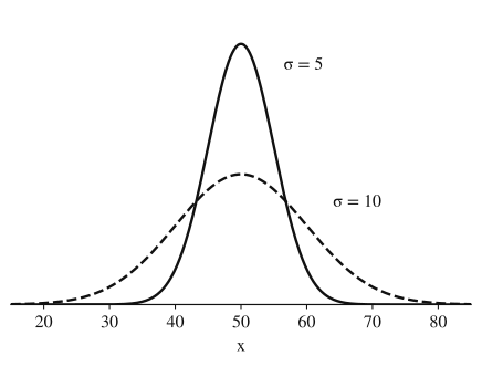
Because the total area must stay 1, spread and height trade off. A smaller $\sigma$ squeezes the area close to the mean, so the curve has to be taller; a larger $\sigma$ spreads it out, so the curve is lower and wider. The figure shows $N(50, 5)$ and $N(50, 10)$: same center, and doubling $\sigma$ halves the height of the peak.

Many variables are well modeled by a normal curve: heights of adults of one sex, weights of manufactured items, measurement errors, standardized test scores. A common reason is that the value is the result of many small, independent influences adding up. Plenty of variables are not normal, though. Incomes, house prices and waiting times are usually skewed right, and a normal model for them gives wrong answers. The normal curve is a model you choose because the data look like it, not a law every variable obeys.

The empirical rule

Every normal curve has the same proportions when you measure distance in standard deviations:

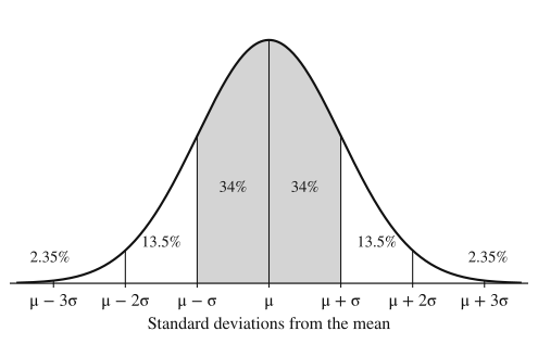
The rule is approximate. The exact area within 2 standard deviations is about 95.45%, and within 1 is about 68.27%. Use the rule when a question says to, or for quick estimates at whole numbers of standard deviations; use technology for anything else.

z-scores and the standard normal distribution

To handle a value that isn't a whole number of standard deviations from the mean, measure its distance in standard deviations exactly. The z-score of a value $x$ is

A loaf of 921 g from $N(900, 15)$ has $z = \frac{921 - 900}{15} = 1.4$: it is 1.4 standard deviations above the mean. Negative z-scores are below the mean.

If $X$ is $N(\mu, \sigma)$, then its z-scores follow the standard normal distribution, $N(0, 1)$: subtracting $\mu$ moves the center to 0, and dividing by $\sigma$ rescales the spread to 1, while the shape stays normal. So one curve, and one table of its areas, answers every normal question. The table on the AP formula sheet gives the area to the left of $z$. On a TI-84, normalcdf(lower, upper, $\mu$, $\sigma$) gives the area between two boundaries without standardizing (use $-1\text{E}99$ or $1\text{E}99$ for an open end).

z-scores also compare relative positions. A value's percentile is the percent of the distribution below it, and in a normal distribution the percentile depends only on $z$. Two values from different normal distributions with the same z-score sit at the same percentile of their own distributions.

From an area back to a boundary

Sometimes the area is given and the boundary is the question: the weight that only the lightest 5% of loaves fall below, or the limits that contain the middle 90%. Find the z-score with that area to its left (invNorm(area, $\mu$, $\sigma$) on a TI-84, or the table read in reverse), then convert back with $x = \mu + z\sigma$. How you assign the area depends on the region:

• Lowest $p$%: the boundary $x_a$ has $P(X < x_a) = \frac{p}{100}$ to its left.
• Highest $p$%: the boundary $x_b$ has $P(X > x_b) = \frac{p}{100}$, so its area to the left is $1 - \frac{p}{100}$.
• Middle $p$%: $P(x_a < X < x_b) = \frac{p}{100}$, with the leftover area split evenly between the two tails.
• Most extreme $p$% (both tails): the $p$% is divided in half, so $P(X < x_a) = \frac{1}{2} \cdot \frac{p}{100}$ and $P(X > x_b) = \frac{1}{2} \cdot \frac{p}{100}$.

The same equation, $x = \mu + z\sigma$, also runs backward to find a parameter. If you know a percentile and one parameter, you know $x$ and $z$, and you can solve for the other one; Example 4 does exactly this.

Worked examples

Where students lose points

On the exam

Normal calculations show up in multiple choice and inside free-response questions, and a calculator is allowed on both sections of the exam, alongside the standard normal table on the formula sheet. Credit for a normal probability requires communication: name the distribution and its parameters, give the boundary and the direction (or a labeled sketch), and state the answer in context. When you work backward to a boundary or a parameter, show the z-score you used and the equation $x = \mu + z\sigma$.