Sampling Distributions and the Central Limit Theorem

A cereal company says 20% of its boxes contain a prize. You buy 50 boxes and find prizes in only 4 of them, a proportion of 0.08. Is the company lying, or did you just get an unlucky set of boxes? You can't answer that from your 50 boxes alone. You need to know what proportions random samples of 50 boxes usually produce when the true rate really is 20%, and that is exactly what a sampling distribution tells you.

A statistic has its own distribution

Topic 2.9 separated a parameter (a fixed number describing a population or distribution, like the true prize rate $p = 0.20$) from a statistic (a number computed from a sample, like the sample proportion $\hat{p} = 0.08$). A parameter has one value. A statistic changes from sample to sample, because each random sample contains different individuals. That variation isn't a flaw in the sampling; it's unavoidable, and it follows a predictable pattern.

The sampling distribution of a statistic is the distribution of its values over all possible samples of the same size $n$ from the same population. It answers the question "if I took every possible sample of this size, what values of the statistic would I get, and how often?"

Keep three distributions apart:

For a tiny population you can list every sample, and Example 1 does. For real populations the number of possible samples is astronomical (there are about $1.6 \times 10^{27}$ ways to choose 20 people from a school of 200), so the sampling distribution is approximated by simulation or described by theory.

Simulating a sampling distribution

To simulate a sampling distribution, you assume a value for the parameter and let a computer play the role of the population:

1. Set up a model of the population with the assumed parameter value (a prize rate of 0.20, say).
2. Draw a random sample of size $n$ from the model and compute the statistic.
3. Repeat step 2 a large number of times, recording the statistic each time.
4. Graph the recorded values. Their distribution approximates the sampling distribution.

For the cereal claim, a computer drew 500 random samples of 50 boxes from a model where each box has a 0.20 chance of a prize, and recorded $\hat{p}$ for each sample:

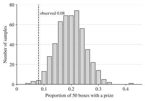
Describe it the way you'd describe any distribution (Topic 1.6): the simulated $\hat{p}$ values are roughly symmetric and unimodal, centered at about 0.20 (the assumed parameter), and mostly between 0.10 and 0.30. Your result, 0.08, sits in the far left tail: only 8 of the 500 simulated samples, $\frac{8}{500} = 0.016$, gave a proportion of 0.08 or lower. If the true rate were 20%, a result this low would happen only about 2% of the time: the simulation estimates 1.6%, and the exact binomial probability (Topic 2.10) of 4 or fewer prize boxes in 50 is $P(X \le 4) \approx 0.0185$. That's convincing evidence that the true prize rate is less than 20%. Unit 3 turns this reasoning into formal hypothesis tests, and Topic 3.2 gives the sampling distribution of $\hat{p}$ a formula.

Randomization distributions for experiments

Experiments need a slightly different simulation, because there's no population to resample. Suppose 10 volunteers are randomly assigned, 5 to chew caffeinated gum and 5 to chew a placebo gum, before a reaction test. Each volunteer's improvement in score is recorded:

The difference in means is $13.4 - 8.0 = 5.4$ points. But the random assignment itself creates differences: even if the gum did nothing, the 5 people who happened to land in one group might improve more. How big a difference does chance assignment alone produce?

Take the 10 improvements exactly as they are, shuffle them, deal 5 to "caffeine" and 5 to "placebo", and compute the difference in means. This reallocation imitates a world where each person's result would have been the same whichever gum they chewed, so any difference comes only from who ended up in which group. Repeat it many times. The distribution of the recorded differences is a randomization distribution, and it approximates the sampling distribution of the difference in means under that no-effect assumption.

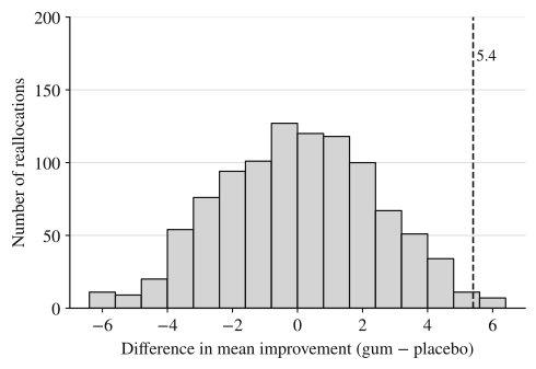
The reallocated differences center near 0, as they should when the gum makes no difference, and only 13 of 1,000 reached 5.4 or more. A difference as large as the one observed is rare from random assignment alone. The simulation puts it at about 1.3% of the time; listing all $\binom{10}{5} = 252$ ways to split the 10 scores into two groups of 5 shows that exactly 4 of them give 5.4 or more, $\frac{4}{252} \approx 1.6\%$. Either way, the experiment gives convincing evidence that the caffeinated gum improved scores for these volunteers.

The central limit theorem

The shape of a sampling distribution depends on the statistic and the population. For the sample mean, one general result describes the shape for almost any population.

Why should averaging produce a bell curve? A sample mean averages $n$ independent values. An unusually large value in a sample is usually offset by ordinary ones, so the extremes of the population rarely survive into the mean, and the many small up-and-down contributions balance out. The figure shows it happening. The population is the time visitors spend on a web page, strongly skewed right with mean 4 minutes and standard deviation 4 minutes. The three histograms each show 10,000 simulated sample means.

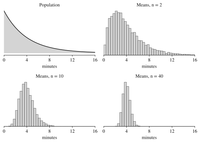
Two more things change as $n$ grows, and both are visible in the figure. The center stays at the population mean, about 4 minutes, for every $n$. The spread shrinks: the simulated standard deviation of $\bar{x}$ is about 2.90 minutes for $n = 2$, 1.27 for $n = 10$ and 0.63 for $n = 40$. Topic 4.1 shows that the standard deviation of $\bar{x}$ is $\sigma/\sqrt{n}$, which here gives 2.83, 1.26 and 0.63 minutes; the simulated values differ from these only by chance variation. The CLT itself is a statement about shape, and only about sample means: it doesn't make the population normal, and it doesn't make the data in your sample normal.

Worked examples

Where students lose points

On the exam

Simulations show up as dotplots or histograms of simulated statistics, usually with the assumed parameter value stated. The questions ask you to describe the simulated distribution, locate an observed statistic in it, compute the proportion of simulated values as extreme as the observed one, and draw a conclusion in context. Central limit theorem questions ask for the shape of a distribution and the reason for it: say which distribution is approximately normal, name the sample size $n$ (or a normal population) as the reason, and keep the population, the sample and the sampling distribution separate.