Electric Fields

Coulomb's law (topic 8.1) gives the force between two specific charges. But a charged object affects every point around it, whether or not another charge is there to feel it, and it is far more useful to describe that effect once, as a property of space, and then get the force on any charge you like by one multiplication. That property is the electric field.

The field as force per unit charge

Charged objects are the sources of electric fields. To measure the field at a point, place a small positive charge $q_0$ there, measure the electric force on it, and divide by $q_0$.

Dividing by $q_0$ is what makes the field a property of the sources rather than of the probe. Double the test charge and the force doubles, so the ratio, the field, stays the same. The idea is the same as the gravitational field near Earth's surface, $g = \frac{F_g}{m} = 9.8\ \text{N/kg}$, which describes Earth's pull on any mass.

A test charge is a point charge small enough that it doesn't disturb the charges producing the field. This matters most near conductors. A large probe charge brought near a charged metal sphere pushes or pulls the sphere's free charge to new places, so it would measure the field of the rearranged sphere, not the field that was there before the probe arrived. The field is defined in the limit of a vanishingly small probe.

Since the definition uses a positive test charge, the field at a point points the way a positive charge there would be pushed. An electron at the same point is pushed the opposite way.

Fields of point charges, added as vectors

Put Coulomb's law into the definition. A test charge $q_0$ at distance $r$ from a point charge $q$ feels a force of magnitude $\frac{1}{4\pi\varepsilon_0}\frac{|q|q_0}{r^2}$, so

A positive test charge is repelled by a positive source and attracted by a negative one, so:

• the field of an isolated positive charge points directly away from it;
• the field of an isolated negative charge points directly toward it.

The field falls as $\frac{1}{r^2}$: at twice the distance it is a quarter as strong.

Fields obey superposition, because forces do. The net field at a point is the vector sum of the fields each source would produce there alone:

For each source, find the magnitude from $\frac{k|q|}{r^2}$ and the direction from its sign (away from $+$, toward $-$), then add components. For example, take $+3.0\ \text{nC}$ and $+1.0\ \text{nC}$ charges $0.20\ \text{m}$ apart. At the midpoint, $0.10\ \text{m}$ from each, the $+3.0\ \text{nC}$ charge makes a field of $2.7\times10^{3}\ \text{N/C}$ pointing toward the $+1.0\ \text{nC}$ charge, and the $+1.0\ \text{nC}$ charge makes $900\ \text{N/C}$ pointing back toward the $+3.0\ \text{nC}$ charge. They point in opposite directions, so the net field is $1.8\times10^{3}\ \text{N/C}$, directed toward the smaller charge.

Topic 8.4 extends the sum to charge spread continuously along a rod or ring, where it becomes an integral.

Picturing the field: vector maps and field lines

A field has a magnitude and direction at every point in space, so drawing it takes a convention. There are two.

A vector field map draws an arrow at each point of a grid. The arrow points along $\vec{E}$ there, and a longer arrow means a stronger field. It is the direct picture of the definition: each arrow is the force per coulomb a positive test charge would feel at that spot. Because a point charge's field grows as $1/r^2$, arrows drawn exactly to scale would be enormous next to a charge and invisible far away, so most maps compress the scale. The map in the figure below does: its arrows are capped in length near the charges and shrink only gradually with distance, so it ranks field strengths correctly but a field ten times stronger does not get an arrow ten times longer.

A field line diagram connects the information into continuous curves, and it is a simplified version of the map. Its rules:

• At every point, the field is tangent to the line through that point, in the direction of the arrowheads.
• Lines begin on positive charges and end on negative charges (or run off to infinity, far from everything).
• The number of lines leaving or entering a charge is proportional to the size of that charge.
• Where lines are close together the field is strong; where they spread apart it is weak.
• Lines never cross: at a crossing the field would have two directions at one point, and the net field has only one.

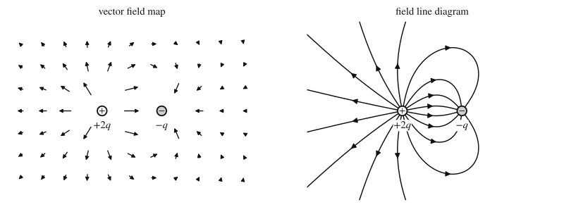
The figure shows both pictures for $+2q$ and $-q$. Twice as many lines leave $+2q$ as end on $-q$, so half of $+2q$'s lines have nowhere to end and head outward: far from the pair, the field looks like that of a single charge $+q$, the net charge. The lines also tell you where the field is weak. Just to the right of $-q$ they spread out and point toward $-q$, while far to the right they point away; in between there is a point where the field is zero (the two fields cancel there, at a distance of about $2.4$ times the charge spacing to the right of $-q$).

Neither picture is the field itself; the field exists at every point, including between the lines. A field line is not the path a charge follows either: a charge's acceleration is along the line, but its velocity need not be.

Fields of charged conductors and insulators

A conductor's free charge can move, and that fixes what its field looks like once everything has settled. A conductor is in electrostatic equilibrium when no charge in it is moving (in metals this takes far less than a microsecond).

• The field inside the material of a conductor is zero. If it weren't, the field would push on the free electrons and they would move, which contradicts equilibrium. The charges rearrange until their own field cancels any field inside.
• Excess charge sits on the outer surface. Like charges repel and spread out as far as they can, which in a conductor means onto the surface. Topic 8.6 proves it with Gauss's law: with $E = 0$ throughout the metal, any closed surface inside the metal encloses zero net charge.
• Just outside the surface, the field is perpendicular to the surface. A component along the surface would push the surface charges sideways, and they would slide until that component vanished.

Insulators behave differently, because their charge can't move. Charge placed on or in an insulator stays where it was put, so excess charge can be spread through the interior as well as on the surface, and the field inside the material is generally not zero. A plastic ball with charge spread uniformly through its volume has a field inside it that grows linearly from zero at the center to its largest value at the surface; topic 8.6 calculates it.

For either kind of object, if the charge is spread with spherical symmetry (the same at every point of each sphere centered on the object), the field everywhere outside it is exactly the field of a point charge equal to the total charge, placed at the center:

A charged metal sphere far from other charges is one example: its charge spreads evenly over its surface, so outside it acts like a point charge, and inside it the field is zero. Topic 8.6 proves the point-charge result, and topic 10.1 develops conductors further.

Worked examples

Worked exampleExample 3: measuring a field to find a charge (free-response style)

A small solid metal sphere of radius $2.0\ \text{cm}$ on an insulating stand carries an unknown charge $Q$. A student mounts a tiny bead with charge $q = +0.50\ \text{nC}$ on an insulating rod attached to a force sensor, holds it at several distances $r$ from the center of the sphere, and records the magnitude of the electric force. The force on the bead points directly away from the sphere at every position.

$r$ (m)	$0.10$	$0.15$	$0.20$	$0.25$	$0.30$
$F$ ($10^{-6}$ N)	$18.3$	$7.9$	$4.4$	$2.9$	$2.0$

(a) The student uses a bead with a much smaller charge than the sphere's. Explain why this is necessary for the measurement to give the sphere's field.

(b) Indicate which quantities should be graphed to give a straight line whose slope can be used to find $Q$. Plot the data and draw a best-fit line.

(c) Use the slope to calculate $Q$, including its sign. Use $k = 9.0\times10^{9}\ \text{N}\cdot\text{m}^2/\text{C}^2$.

(d) Calculate the electric field at $r = 0.20\ \text{m}$ from the data, and state the field at $r = 1.0\ \text{cm}$ from the center. Justify the second answer.

Show solution

(a) The sphere is a conductor, so its charge can move. A bead with a large charge would attract or repel the sphere's charge toward or away from it, changing the field it is trying to measure. A bead with a small charge is a test charge: it leaves the sphere's charge distribution, and so the field, essentially unchanged.

(b) The sphere's charge is spread evenly over its surface, so outside it the field is that of a point charge at its center, and the force on the bead is $F = \frac{kQq}{r^2}$. Graphing $F$ against $\frac{1}{r^2}$ should give a straight line through the origin with slope $kQq$. The values of $\frac{1}{r^2}$ are $100$, $44.4$, $25.0$, $16.0$ and $11.1\ \text{m}^{-2}$.

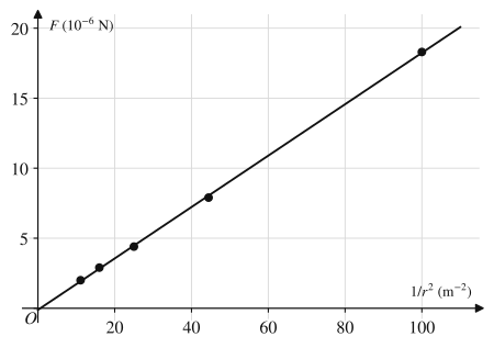
(c) The best-fit line passes near the origin and through points such as $(100\ \text{m}^{-2},\ 18.2\times10^{-6}\ \text{N})$, so its slope is about

$$\text{slope} = \frac{18.2\times10^{-6}\ \text{N}}{100\ \text{m}^{-2}} = 1.8\times10^{-7}\ \text{N}\cdot\text{m}^2.$$

Setting slope $= kQq$,

$$Q = \frac{\text{slope}}{kq} = \frac{1.8\times10^{-7}\ \text{N}\cdot\text{m}^2}{(9.0\times10^{9}\ \text{N}\cdot\text{m}^2/\text{C}^2)(0.50\times10^{-9}\ \text{C})} = 4.0\times10^{-8}\ \text{C} = +40\ \text{nC}.$$

$Q$ is positive because the positive bead is repelled. Using the slope instead of a single data point averages out the scatter in the measurements.

(d) At $r = 0.20\ \text{m}$,

$$E = \frac{F}{q} = \frac{4.4\times10^{-6}\ \text{N}}{0.50\times10^{-9}\ \text{C}} = 8.8\times10^{3}\ \text{N/C},$$

directed away from the sphere (the force on a positive test charge points along the field). At $r = 1.0\ \text{cm}$ the point is inside the metal of the sphere, and the field there is zero. The sphere is a conductor in electrostatic equilibrium: any field inside the metal would push its free electrons and they would still be moving.

Where students lose points

On the exam

Field questions come as calculations of $\vec{E}$ from up to a few point charges (magnitude and direction), as comparisons ("rank the field magnitudes at points A, B and C" from a field-line diagram, using line density), and as experimental design and analysis: choosing what to measure, linearizing data like Example 3, and extracting a charge or field from a slope. When you justify a direction, name the source's sign. When you justify $E = 0$ inside a conductor, say that a nonzero field would move the free charges, contradicting equilibrium.