Electric Potential

The potential energy of topic 9.1 depends on two things at once: the charges that set up the field and the charge you bring into it. Divide out the charge you bring in and what is left describes the location alone, the way the field $\vec{E} = \frac{\vec{F}}{q}$ describes the force per unit charge at a point. That quantity is the electric potential. It is a scalar, so it is usually easier to compute than the field, and the field can be recovered from it by differentiating.

Potential is energy per unit charge

Place a small test charge $q$ at a point P near some fixed charges. The system's potential energy from the test charge's interactions with them is $U_E$. The electric potential at P is

Doubling $q$ doubles $U_E$, so $V$ does not depend on the test charge at all; it is set by the other charges and the location. Its unit is the volt: $1\ \text{V} = 1\ \text{J/C}$.

What gets measured in practice is the potential difference between two points. Moving a test charge from A to B changes the system's energy by $\Delta U_E$, and

Turned around, $\Delta U_E = q\,\Delta V$. Positive charge gains potential energy moving to higher potential; negative charge loses it. Topic 9.3 builds on that relation.

Dividing topic 9.1's two-charge energy by the test charge gives the potential of a single point charge $q$ at distance $r$, and because energies of separate pairs add, potentials from separate charges add too.

For example, $+4.0\ \text{nC}$ sits at the origin and $-2.0\ \text{nC}$ at $(0.30\ \text{m}, 0)$. Point P at $(0, 0.40\ \text{m})$ is $0.40\ \text{m}$ from the first charge and $0.50\ \text{m}$ from the second (a 3-4-5 triangle), so

A $-1.5\ \text{nC}$ charge placed at P would add $U_E = qV_P = (-1.5\times10^{-9})(54) = -8.1\times10^{-8}\ \text{J}$ to the system's energy, the sum of its two new pair energies in one step.

Batteries. Potential differences don't only come from charges set out on purpose. In a battery, chemical reactions push positive charge toward one terminal and negative charge toward the other, against the electric force that would pull them back together. The separated charge holds the terminals at different potentials: an alkaline cell keeps its positive terminal about $1.5\ \text{V}$ above its negative one, so every coulomb that goes through the external circuit from one terminal to the other can deliver about $1.5\ \text{J}$. Unit 11 uses this as the battery's emf.

Potential from the field

When a test charge moves a small displacement $d\vec{\ell}$, the field does work $q\vec{E}\cdot d\vec{\ell}$ on it, and the system's potential energy changes by the negative of that. Divide by $q$ and add up the steps:

Three consequences follow immediately.

• Uniform field. Moving a distance $d$ in the direction of $\vec{E}$, $\Delta V = -Ed$. Moving perpendicular to $\vec{E}$, $\Delta V = 0$. So $1\ \text{V/m} = 1\ \text{N/C}$, and a field of $2000\ \text{V/m}$ drops the potential by $20\ \text{V}$ every centimeter you move along it.
• Point charge. Integrate inward from $\infty$, where $V = 0$, along a radial line: $V(r) = -\int_\infty^r \frac{q}{4\pi\varepsilon_0 r'^2}\,dr' = \frac{q}{4\pi\varepsilon_0 r}$, the formula above.
• Infinite line of charge, or outside a long charged cylinder. Gauss's law (topic 8.6) gives $E = \frac{\lambda}{2\pi\varepsilon_0 r}$, radially outward for $\lambda > 0$. Integrating from a reference distance $r_0$ to $r$:

Here you cannot put the zero at infinity: $\ln\frac{r}{r_0}$ grows without limit as $r \to \infty$, because an infinitely long line carries infinite charge. Only differences are meaningful, or you pick a finite reference distance where $V = 0$. For a line with $\lambda = 5.0\ \text{nC/m}$, going from $2.0\ \text{cm}$ to $8.0\ \text{cm}$ from it changes the potential by $-\frac{\lambda}{2\pi\varepsilon_0}\ln 4 = -(2)(9.0\times10^{9})(5.0\times10^{-9})(1.386) = -125\ \text{V}$.

Potential of a continuous charge

For charge spread along a line or over a surface, split it into pieces $dq$, treat each as a point charge, and add:

where $r$ is the distance from each piece to the point. Compared with the field integrals of topic 8.4, this is easier: there are no components to project and no cancellations to argue. The course limits the potentials you must find by integration to four objects, each at particular points:

A ring on its axis. Every piece of a ring of radius $R$ and charge $Q$ is the same distance $\sqrt{R^2 + z^2}$ from a point at height $z$ on the axis, so that distance comes out of the integral:

An arc at its center. Every piece of a semicircle, or any part of a circle, is the distance $R$ from the center, so $V = \frac{1}{4\pi\varepsilon_0}\frac{Q}{R}$, with $Q$ the charge on the arc. This holds even if the charge is spread unevenly along the arc. The field at the center does depend on how the charge is spread, because there the directions matter.

A finite rod on its perpendicular bisector. A rod of length $L$ with uniform $\lambda$ lies along the $x$-axis from $-\frac{L}{2}$ to $\frac{L}{2}$. A piece $dq = \lambda\,dx$ is $\sqrt{x^2 + y^2}$ from the point $(0, y)$:

using $\int\frac{dx}{\sqrt{x^2 + y^2}} = \ln\left(x + \sqrt{x^2 + y^2}\right)$. Example 3 does the rod's other case, a point on the rod's own line.

An infinite line or cylinder at a distance is easiest from its field, as in the previous section.

A good check on any of these: far away, the object looks like a point, so $V$ must approach $\frac{Q}{4\pi\varepsilon_0 r}$. The ring passes, since for $z \gg R$ the square root is about $z$.

Field from potential, and equipotentials

Run the integral backward. For a small step $dx$ along the $x$-axis, $dV = -E_x\,dx$, so:

On a graph of $V$ against $x$, $E_x$ is the negative of the slope. Where the graph rises, $E_x < 0$; where it is flat, $E_x = 0$, whatever the value of $V$ there. For the ring, differentiating its axial potential gives the axial field in one line,

the same result topic 8.4 gets by integrating components.

An equipotential (or isoline, in two dimensions) is a line or surface on which $V$ has one value. A map of them is like a contour map of a hillside, with potential in place of height.

• Equipotentials are perpendicular to the field. Moving along one, $\Delta V = 0$, so $\vec{E}\cdot d\vec{\ell} = 0$: the field has no component along an equipotential.
• The field points from higher to lower potential, crossing the lines at right angles, like the steepest way down a hill.
• Crowded lines mean a strong field. If lines are drawn at equal steps $\Delta V$, the field near them has magnitude about $\frac{\Delta V}{\Delta s}$, where $\Delta s$ is the spacing.
• Either map gives the other. From field arrows, draw lines crossing them at right angles. From equipotentials, draw arrows perpendicular to them, pointing toward the lower values.

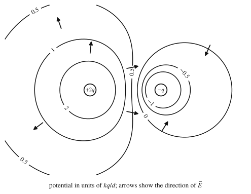
The map tells you how charges will move. A positive charge is pushed along $\vec{E}$, toward lower potential; a negative charge is pushed the other way, toward higher potential. Carrying any charge along an equipotential takes no work. Topic 10.1 adds that the surface of a conductor in equilibrium is an equipotential.

Worked examples

Worked exampleExample 2: from a graph of V to the field

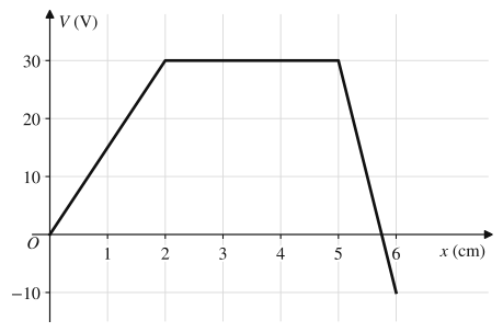
The graph shows the electric potential along the $x$-axis in a region where the field points along the axis.

(a) Calculate $E_x$ in each of the three regions.

(b) Describe the graph of $E_x$ against $x$ from $0$ to $6\ \text{cm}$.

(c) An electron is at $x = 1.0\ \text{cm}$. Calculate the electric force on it, with direction.

(d) Calculate the work done by the electric field on an electron that moves from $x = 0$ to $x = 6.0\ \text{cm}$. The electron charge is $-1.60\times10^{-19}\ \text{C}$.

Show solution

(a) Use $E_x = -\frac{dV}{dx}$; each region is a straight line, so the derivative is the slope. Convert centimeters to meters.

• $0$ to $2\ \text{cm}$: slope $\frac{30\ \text{V}}{0.020\ \text{m}} = 1500\ \text{V/m}$, so $E_x = -1500\ \text{V/m}$ (the field points in the $-x$ direction).
• $2$ to $5\ \text{cm}$: slope zero, so $E_x = 0$, even though $V = 30\ \text{V}$ there.
• $5$ to $6\ \text{cm}$: slope $\frac{-40\ \text{V}}{0.010\ \text{m}} = -4000\ \text{V/m}$, so $E_x = +4000\ \text{V/m}$.

(b) A step graph: a horizontal segment at $-1500\ \text{V/m}$ from $0$ to $2\ \text{cm}$, zero from $2$ to $5\ \text{cm}$, and $+4000\ \text{V/m}$ from $5$ to $6\ \text{cm}$, with jumps at $2\ \text{cm}$ and $5\ \text{cm}$. The field is strongest where the $V$ graph is steepest. Note that at $x = 5.75\ \text{cm}$, where $V = 0$, the field is $4000\ \text{V/m}$.

(c) $F_x = qE_x = (-1.60\times10^{-19}\ \text{C})(-1500\ \text{V/m}) = +2.4\times10^{-16}\ \text{N}$, in the $+x$ direction: opposite to the field, toward higher potential, as it must be for a negative charge.

(d) The field's work is the negative of the change in potential energy, $W = -q\,\Delta V$, and only the endpoints matter:

$$W = -(-1.60\times10^{-19}\ \text{C})(-10\ \text{V} - 0) = -1.6\times10^{-18}\ \text{J}.$$

The electron ends at lower potential than it started, which for a negative charge means higher potential energy, so the field did negative work overall.

Where students lose points

On the exam

Potential questions ask you to add point-charge potentials, set up and evaluate $\int\frac{dq}{r}$ for the four shapes listed above, get $\Delta V$ from a field (integrating, or $Ed$ in a uniform field), get $E_x$ from a $V$ graph or expression, and translate between field-vector maps and equipotential maps. When you sketch $E_x$ from a $V$ graph, show the sign: the value is the negative slope, segment by segment. When a question asks for the potential at a point, state the reference you used (zero at infinity unless the object is infinitely long).